β^- Decay Half-Lives: A Global Model With Neural Networks [upper part]

NNs are structures, inspired from the corresponding biological neural systems, that consist of interconnected processing units (called neurons) arranged in a distinct layered topology. In analogy to the biological neural structures, the function of the network is determined from the connections between the units. Topology and connections determine the architecture of a network.

Static Feedforward Neural Networks (NNs), with strictly forward connections, often have one or more intermediate hidden layers of nonlinear processing units, followed by an output layer of linear units. Such an architecture may be summarized in the notation:

where I is the number of inputs, Hi is the number of neurons in the ith hidden layer, O is the number of units in the output layer and C is the total number of connections (known as synaptic weights or just weights) and biases.

The connection from neuron i to neuron j is characterized by a real number weight wij. The output ai of neuron i is transmitted through this connection to neuron j and multiplies its strength by the weight wij, forming accordingly the weighted input wijai. Each neuron has additionally a bias b which is summed with its weighted inputs to form its net input. This quantity feeds the activation function f that produce the output aj of neuron j.

Given two set of data, input/output pairs, NNs are able to learn a specific nonlinear mapping by adjusting the network weights and bias by using the training algorithm (see Machine Learning Procedure). The goal of network training is not to learn an exact representation of the known halflives itself, but rather to build a statistical model of the process which generates the half-lives. This is very important for a good generalization and leads to a reliable statistical model. The mostly used training algorithm is the back-propagation (BP) algorithm in many variations, where a steepest descent gradient approach and a chain-rule are adopted for back-propagating the error correction from the output layer. The initial values of the free parameters (weights and biases) play also a crucial role in the final result. After a large number of computer experiments, we reach a model suitable to both approximate the observed β- decay half-life systematics and to generalize well to unknown regions. The main features of our model are recapitulated in the table below.

N. J. Costiris(1), E. Mavrommatis (1), K. A. Gernoth (2) and J. W. Clark (3)

(1) Physics Department, Division of Nuclear and Particle Physics, University of Athens, GR-15771 Athens, Greece

(2) Department of Physics, UMIST, P.O. Box 88, Manchester M60 1QD, United Kingdom

(3) McDonnell Center for the Space Sciences and Department of Physics, Washington University, St. Louis, Missouri 63130, USA

Statistical modeling of nuclear data provides a novel approach to nuclear systematics which valuably complements the phenomenological and semi-microscopic theories. Currently, there is an urgent need for reliable estimates of β- decay halflives of nuclei far from stability. This need is driven both by the experimental programs of existing and future radioactive ion-beam facilities and by ongoing major efforts in astrophysics toward understanding supernova explosions, and the processes of nucleosynthesis in stars, notably the r-process. In this work, the beta decay halflives problem is dealt as a many-body system optimization problem, which is resolved in the statistical framework of machine learning. Continuing past similar approaches, we deploy a more sophisticated Artificial Neural Networks (NNs) statistical methodology to global model the halflives systematics of nuclei that decay 100% by the β- mode in their ground states. A fully connected, static, multilayered feedforward neural network NN was adopted and trained using the Levenberg-Marquardt optimization algorithm with a combination of two well-established techniques for improving generalization, namely, Bayesian regularization and cross-validation. We report here our methodology for the arising large-scale calculations and discuss and compare our results with the available experimental [7], the theoretical ones and some other results obtained with analogous techniques (previous ANNs and more recent Support Vector Machines (SVMs) approaches). We then give predictions for nuclei that are far from the stability line and focus in particularly to those involved in the r-process nucleosynthesis. It seems that our new statistical “theory-thin” data-driven global model can at least match or even surpass the predictive performance of the best conventional “theory-thick” theory-driven global models.

Introduction

Main β-Decay Global Models

Machine Learning Procedure

Results

Several models for determining β- halflives have been proposed and applied during the last few decades. These include the more phenomenological models based on Gross Theory (GT) [1], as well as models (in various versions) that employ the Quasiparticle Random-Phase Approximation (QRPA) [2,4], along with some approaches based on shell-model calculations. The latest version of the RPA models developed by Möller and coworkers, combines the pn-QRPA model with the statistical Gross Theory of ff-decay [3,11]. There are also some models in which the ground state of the parent nucleus is described by the extended Thomas-Fermi plus Strutinsky integral method or the Harrtre-Fock BCS and which the use the continuum QRPA (CQRPA) [5]. Recently a relativistic pn-QRPA (RQRPA) model has been applied in the treatment of neutron-rich nuclei in the N = 50 and 82 regions [6].

Machine learning statistical framework

target

(Log10Tβ,exp)

Output

(Log10Tβ,calc)

input

[Z,N,δ]

Machine:

Neural Network

with C weights

weights adjustment

comparison

Objective: The minimization of the cost function ED

The Levenberg - Marquardt update rule (LM algorithm)

where w represents the vector of weights, J is the Jacobian matrix that contains first derivatives of the machine errors with respect to the weights, I is the unit matrix, μ is an adjustable parameter that controls the step size and e is a vector of network errors. The central idea of learning machines is that the free parameters (weights) can be adjusted by minimizing the cost function (ED ) through a proper training algorithm (LM for example), so that the machine responds to a desired behavior.

Data Sets

Our β- Decay Global Model [8]

Comparison With Theory Thick Global Models

Comparison With Experiment

The partitioning of NuSet-B with a cutoff at 106 sec

into the three subsets: Learning,

Validation and Test Sets

NuSet-B consists of 838 nuclides: 503 (~60\%) of them have been uniformly chosen to train the network (learning set), 167 (~ 20\%) to validate the learning procedure (validation set) and the remaining 168 (~ 20\%) to evaluate the accu-racy of the prediction (test set). With the exclusion of the long-lived examples (>106s), one is dealing with a smaller but more homogeneous collection of nucli-des that facilitates the training of the network. From now on we will refer to the whole set of 838 nuclides with the term Overall Mode and to the test set of 168 nuclides (that tests the extrapability of the model) with the term Prediction Mode.

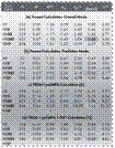
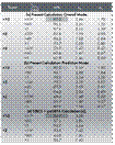
The above Fig. illustrates present calculations of β-decay half-lives in comparison with experimental values for nuclides in the learning, validation and test sets.

Theory

Thick

Global

Models

[1-6]